Excel – Conditional Formatting with Subtotals
Microsoft Excel, Microsoft Office
If there has ever been a more “You’ve got your chocolate in my peanut butter!” moment, it’s the blending of Conditional Formatting with the Subtotals tool in Excel.
If you have ever used the Subtotals tool to group information you have probable been impressed with its ability to group data by some changing event (like States) and have those groups aggregated and then structured into a collapsible outline.
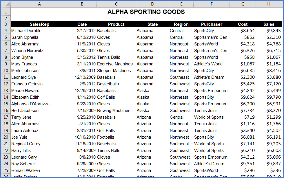
Before Subtotals
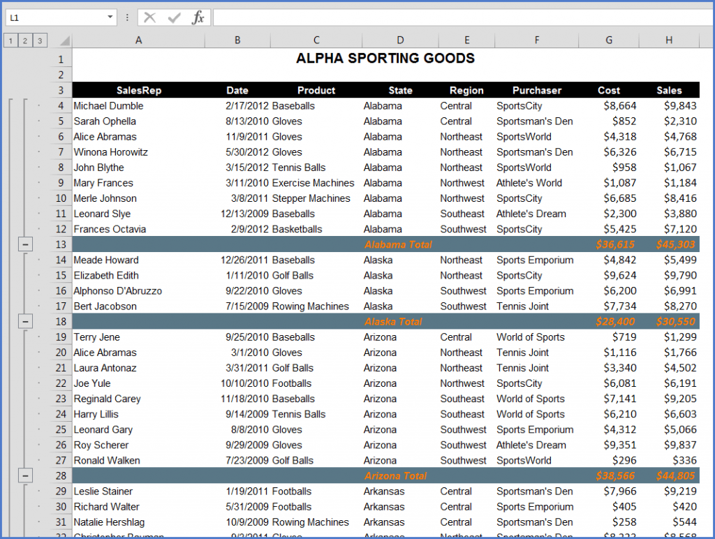
After Subtotals
But the one shortfall when it comes to the Subtotals tool is that there are no built-in artistic styles that can be applied to give the list a bit of pizazz.
You could try to convert the list to a Data Table, but that tool is really meant for straight tables with no intermediate calculations.
CONDITIONAL FORMATTING TO THE RESCUE!!!!!!!!!!!
A common request among Excel users is to have the Subtotal lines be filled with a color to help identify them with greater ease. Conditional Formatting is so versatile when painting data based on some criteria, it becomes a perfect tool for achieving just the desired look. Here are the steps:
Step 1: Selecting the Data Range
Highlight all of the columns containing data. In the above example, that would be Columns “A” through “H” (A:H). This is a good strategy when you are unsure as to the number of records contained in the data. If you wish to be a bit more conservative with memory management, select a range of cells that you are sure you will never exceed (i.e. A4:H1000).
Step 2: Create a New Conditional Format Based on a Formula
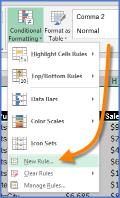
On the Home tab, click the Conditional Formatting button and select New Rule…
The formula needed to achieve the highlight effect is as follows:
=ISNUMBER(SEARCH(“Total”,$D1))
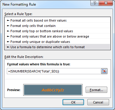
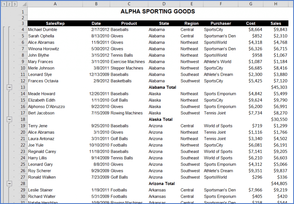
The purpose of this formula is to search for the word “Total” in the text contained in Column “D”. If it finds the word “Total”, it will return the character position of the word within the text (i.e. “9” in the case of “Alabama Total”).
The ISNUMBER function then checks to see if a number was discovered (the word “Total” exists) or an error was returned (“#VALUE” if the word “Total” was not found). This generates a “True/False” response that is passed to the Conditional Formatting tool.
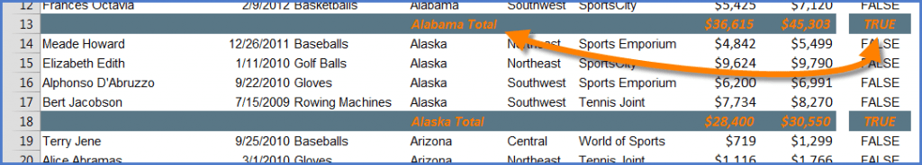
Since every cell in the selected range is looking at its Column “D” position, every cell on a row containing the word “Total” will receive the new formatting instruction.
Step 3: Apply Color Scheme
This step is all about making the cell the color(s) that looks best for the report and the tastes of the designer and viewer.