Excel – Hide Records with Zeroes in Pivot Table Calculations

Microsoft Excel, Microsoft Office

One of the most asked questions of beginning, and sometimes seasoned, pivot table users is “How do I hide the entries in a pivot table whose totals equal zero?”  On first blush, this seems like an easy feat, but users quickly discover that it’s not as easy as predicted.  There are ways to sort the source data and then exclude the entries with zero values, but that task of sorting and filtering the source data would have to be performed each time the source data is updated.  This is not an appealing prospect.

There is actually a very easy way to not display pivot table records that equal zero.

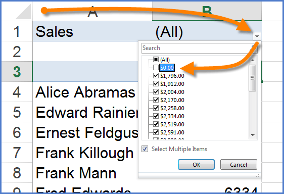
The trick is to add the field that is located in the VALUES section of the pivot table to the FILTERS section as well.

This will not remove the field from the VALUES section but instead give you the ability to filter based on that same information.

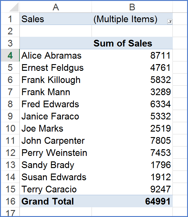
By selecting the filter control for the FILTERS field at the top of the pivot table, you can now deselect zero from the list of displayable items and the problem is solved.