Excel Lookup with Dynamic Input

Microsoft Excel, Microsoft Office

VLOOKUP is great for returning information from a database, but one of the limitations is that the return information is static.

What if the user wishes to look for certain data one day but different data another day?  This would require either two different sets of VLOOKUP functions or the functions would need to be reprogrammed.

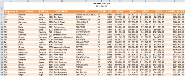
In the database below, the user would wish to return address information in one scenario, but return financial information in another scenario.

Suppose there are times when the user requires a mixture of the two; that would require a third set of VLOOKUP functions. This could become an ever evolving set of work.

ORIGINAL DATABASE

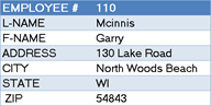
ADDRESS INFORMATION

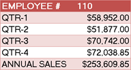
FINANCIAL INFORMATION

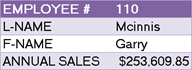
MIXED INFORMATION

Here comes MATCH to the rescue!!!

The MATCH function’s job is to return the relative position of data within a defined array.

The syntax for the MATCH function is:

=MATCH(Lookup_value,Lookup_array,Match_type)

• Lookup_value – The value that you want to find in the list of data. This argument can be a number, text, logical value, or a cell reference.
• Lookup_array – The range of cells being searched.
• Match_type (optional) Tells Excel how to match the Lookup_value with values in the Lookup_array. Choices: -1, 0, or 1. The default value for this argument is 1.
  • If the Match_type = 1 or is omitted: MATCH finds the largest value that is less than or equal to the Lookup_value. The Lookup_array data must be sorted in ascending order.
  • If the match_type = 0: MATCH finds the first value that is exactly equal to the Lookup_value. The Lookup_array data can be sorted in any order.
  • If the Match_type = -1: MATCH finds the smallest value that is greater than or equal to the Lookup_value. The Lookup_array data must be sorted in descending order.

If we wish to give the user the ability to dynamically select which fields of interest to return information from, the MATCH function can examine the category for each row (or column) and use it to calculate the position of that choice in the database.

That position number can then be used for the VLOOKUP Col_Index_Num variable.

*** Remember – VLOOKUP has the following syntax: ***

Let’s look at a VLOOKUP from the static ADDRESS INFORMATION table (FYI: The above database which occupies range $A$5:$L$29 has been given a NAMED RANGE of “Database1”)

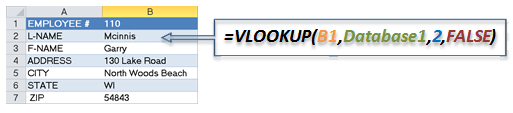
The “2″ in the third variable position is telling us to return data from the 2^nd relative column position from within the table (in this case, Column “B”).

We can calculate that position with the following MATCH function (FYI: The database’s header row which occupies range $A$4:$L$4 contains all of the category names and has been given a NAMED RANGE of “Categories“)

=MATCH(A2,Categories,0)

If we execute this function by itself, it would return “2″ as an answer, since “L-Name” exists in the 2^nd column of the database.

Now we’ll substitute the original “2″ in the Col_Index_Num variable with the MATCH function:

=VLOOKUP(B1,Database1,MATCH(A2,Categories,0),FALSE)

*** IMPORTANT ***

The categories that the user types in Column “A” (in the above example) MUST match the names used in the database header row.

Let’s add some pizzazz to this process

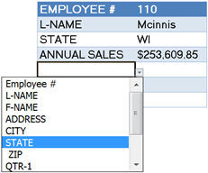
Since a requirement of the MATCH function is we use the same naming convention as the database, and the database contains all of the names, let’s use those names in a dropdown list so the user can select items with greater ease and precision.

This can be accomplished by use of the Data Validation tool.

If we define a report area large enough to display all of a record’s information (accommodate the maximum number of return items), what happens when a user does not use all of the slots?

Any place a category is not defined, a “#N/A” error message will appear.  By placing all of the above VLOOKUP logic inside of an IFERROR function, we can suppress the “#N/A” error messages.

The blanks are generated by means of two double quotation marks placed side by side (no space between them).

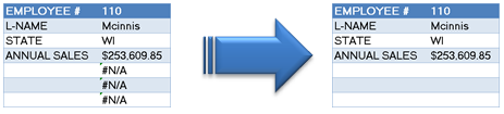
=IFERROR(VLOOKUP(B1,Database1,MATCH(A2,Categories,0),FALSE),””)

BONUS TRICK

If your dataset had non-user friendly headers, you could get fancy and have a table of official headings/user friendly headings and nest another VLOOKUP in the Lookup_Value variable position.

This would allow you to have understandable choices in your data validated dropdown list, but still find the correct category in the less friendly database headings.

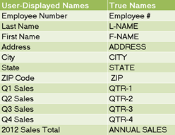
The table above was given the name “NewHeader”

=VLOOKUP(B1,Database1,MATCH(VLOOKUP(A2,NewHeader,2,False),Categories,0),FALSE)