Excel – Mixed Pivot Table Layout

Microsoft Excel, Microsoft Office

Excel – Mixed Pivot Table Layout

Microsoft Excel Pivot Tables is one of the greatest inventions known to man; second only to those buttery mints they bring you in fancy restaurants.  Even the greatest of ideas are not without their issues.  Take for example the Report Layout feature in Pivot Tables.  Excel gives the user three options with which to display hierarchically (wow; that’s a hard word to spell) related data.

• Compact Form
• Outline Form
• Tabular Form

Let’s examine what makes each layout unique.

Compact Form

All row-based data is combined into a single column, one row per line item, and indented to reflect the position within the hierarchy.

Outline Form

All row-based data is separated into individual columns to reflect the position within the hierarchy, one row per line item.

Tabular Form

All row-based data is separated into individual columns to reflect the position within the hierarchy, and the entire hierarchy is placed on a single row (one row per child item.)

While these report layouts are all well and good, suppose you want a combination of layouts in your pivot table?

Report Requirement

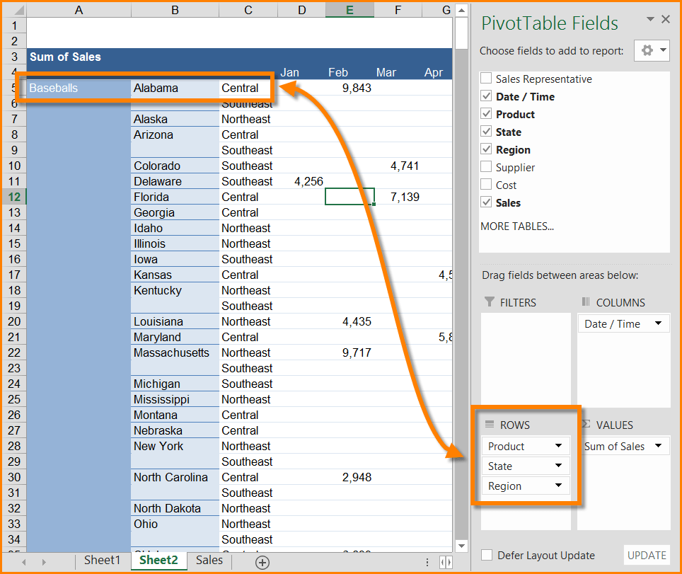
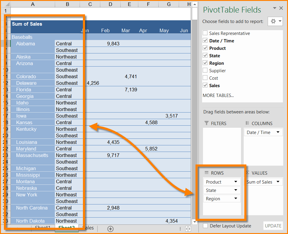
In order to maximize screen space, the developer wants to have the first two levels of the hierarchy (Product and State) in one column and the child level (Region) in a separate column.

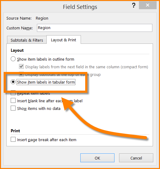
The trick is to select the Compact Form for the pivot table.  In order separate the children (Regions) from the column, click on the State entry in the ROWS section and select Field Settings…

In the Field Setting Dialog Box, select “Show item labels in tabular form” and click OK

You can now sit back and admire you creation.