Excel Pivot Tables Filter by Values

Microsoft Excel, Microsoft Office

If you’ve ever used Pivot Tables in Excel, you no doubt have discovered the wonders of filtering.  The ability to filter row or column items can be extremely helpful when you don’t wish to analyze all of the items in the driving data set.

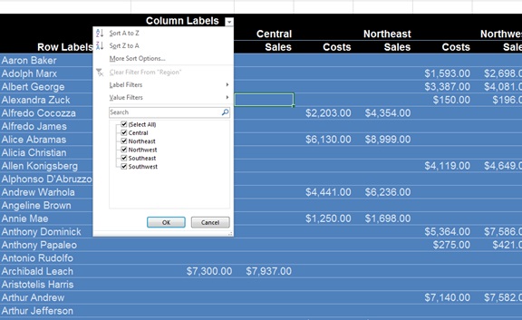
But what do you do if you wish to filter by the Value-based items?  In other words, the numbers in the “connect the dots” area where row and column choices intersect.  These, on first glance, don’t appear to have sorting and filtering controls available.

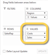
Rest assured, they do exist; you just have to dig a bit to find them.

If you right-click on any row-based item, the following menu will appear.

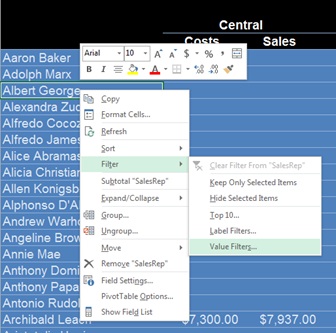
From here, you can filter by any of the traditional controls:

Top 10

• Filter in either direction. Top or Bottom
• Filter the target by any Value-based entry (ex: Cost or Sales)
• Filter by Item count from 1 to the maximum item count in your data set
• Filter by Percentage from 0% to 100%
• Filter by Sum from 1 to the maximum sum in your data set

Label Filters

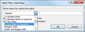
Filter the selected column by any text or date criteria (depending on the nature of the data) with the obligatory text-based or date-based filters (i.e. Greater Than, Less Than, Contains, Begins With, etc…)

Value Filters

Filter the data by the selected Value-based entry (ex: Sales or Cost) with any of the obligatory value-based (i.e. Equal to, Greater Than, Less Than, Is Between, etc…)

Bonus Tip

Another nice trick is to select row entries (via the traditional CTRL-Click or Click-Shift-Click selection techniques) and then Right-click on one of the selected items and choose:

• Keep Only Selected Items
• Hide Selected Items

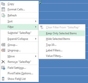
This allows you to quickly reduce a long list to a short list without the need to check and uncheck a series of tiny boxes.