Using Excel MODE Function to Return a Text Response

Microsoft Excel, Microsoft Office

Excel’s MODE function is a great tool for returning the most frequently occurring number in a set of numbers.  But what if you want to return the most frequently occurring word in a list of words?

MODE with Numbers

Using the MODE function in Excel is quite simple; you point to a list of numbers and MODE will tell you which number occurs the most often.

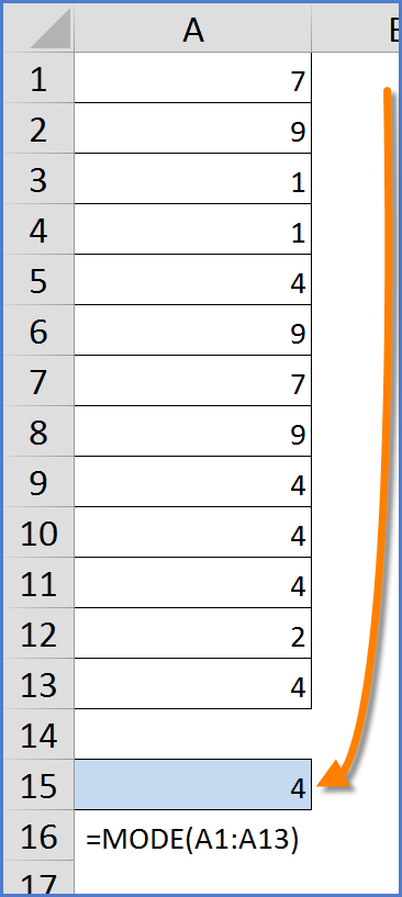
In this list, the number “4” appears more often than any other number.

MODE with Words

As you can see, the MODE function does not work very well when pointing to a list of words.

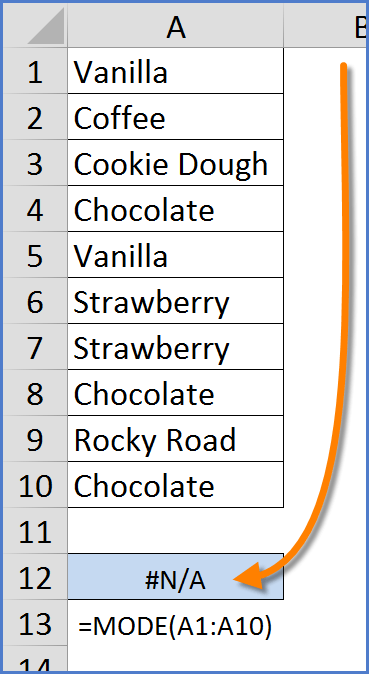
The function returns a “#N/A” error message.

Not to fear; MODE can be made to return words, but it take the combined efforts of SEVERAL functions, none of which are MODE!  (How odd does THAT sound?)

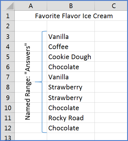
To set the stage, I have created a list of answers to the question, “What is your favorite flavor of ice cream?”  I have named this range of 10 responses “Answers”.  This will make the formulas a lot prettier.

There are four steps required to compute the final answer.  Let’s take them one step at a time.

NOTE:  Each of these formulas must work with the data in an array format.  Therefore, a CTRL-SHIFT-ENTER is required when finalizing each step.  Color-coding has been used to help identify the steps within the steps.

Step 1

{=COUNTIF(Answers,Answers)}

Yields: {2;1;1;3;2;2;2;3;1;3}

This step takes each flavor and counts the number of time that flavor appears in the entire list of answers.

Step 2

{=MAX(COUNTIF(Answers,Answers))}

Yields: 3

This is the number that occurs most frequently in the list generated by Step 1.

Step 3

{=MATCH(MAX(COUNTIF(Answers,Answers)),COUNTIF(Answers,Answers),0)}

Yields: 4

This is the position in the list of answers where the first instance of MAX (i.e. 3) occurs.

Step 4

{=INDEX(Answers,MATCH(MAX(COUNTIF(Answers,Answers)),COUNTIF(Answers,Answers),0))}

Yields: “Chocolate”

This is the text in the 4th position in the list of Answers.

The Finished Formula

So the finished formula reads as follows:

{=INDEX(Answers,MATCH(MAX(COUNTIF(Answers,Answers)),COUNTIF(Answers,Answers),0))}

As you can see from the table below which uses a simple COUNTIF function to count the number of times each flavor occurs in the list, “Chocolate” appears more often than any other flavor.

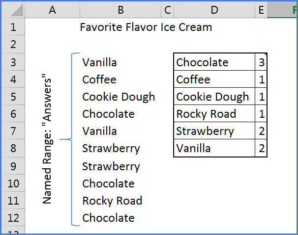
Our super-formula will return the word “Chocolate” as opposed to the number 3.

DON’T FORGET!!!!  These are array formulas and require the use of CTRL-SHIFT-ENTER when committing to the cells.