Excel Hidden Camera Tool – Great for Dashboards

If you are an Excel user who likes to create charts, design dashboards, or just likes to play with neat toys in Excel, this tutorial is going to be right up your alley.

Excel contains (in a super-secret place) a hidden camera.  “But why would I need a hidden camera in a spreadsheet program?”  I’m glad you asked.  If you have ever created a chart on one sheet, but you need the chard displayed simultaneously on a different sheet, and you don’t want to make two of the same thing, the camera tool will solve this problem.

First thing’s first; we have to find the camera before we can put it to creative use.

Read More

12 Excel Keyboard Shortcuts for Every User

Keyboard shortcuts are a great way to improve the speed at which documents are built, regardless of the application.  It seems like there is a keyboard shortcut for just about every feature Excel contains; and there may be that one guru in the office that knows them all.  But most of us fall somewhere between Guru and Labrador retriever (hopefully, closer to the former.)

The good news is that it’s not an “all or nothing” proposition when it comes to keyboard shortcuts.  Knowing just a few of the most productive keyboard shortcuts will serve you far better than knowing none at all.

So let’s get this show on the road!

  1. CTRL+SHIFT+L – Turn On/Off Filter Controls

Filters are of tremendous use when analyzing large numbers of records in a table, but you are only interested in a select set of records that met a specific criteria.  Activating your filters is just a CTRL-SHIFT-L away.  This keyboard can also be used to turn off all of the filters and display the entire list.  (Filters are on by default when you convert a straight table to a Data Table, and not always desired.)  Finally, if you hit the “L” key twice (CTRL-SHIFT-L & L) you can effectively clear the current filters to start fresh with a new filter query.

Read More

Excel – Conditional Formatting with Subtotals

If there has ever been a more “You’ve got your chocolate in my peanut butter!” moment, it’s the blending of Conditional Formatting with the Subtotals tool in Excel.

If you have ever used the Subtotals tool to group information you have probable been impressed with its ability to group data by some changing event (like States) and have those groups aggregated and then structured into a collapsible outline.

Before Subtotals

CondFmt1

After Subtotals

CondFmt2

But the one shortfall when it comes to the Subtotals tool is that there are no built-in artistic styles that can be applied to give the list a bit of pizazz.

Read More

Using Excel MODE Function to Return a Text Response

Excel’s MODE function is a great tool for returning the most frequently occurring number in a set of numbers.  But what if you want to return the most frequently occurring word in a list of words?

MODE with Numbers

Using the MODE function in Excel is quite simple; you point to a list of numbers and MODE will tell you which number occurs the most often.

Mode1

In this list, the number “4” appears more often than any other number.

MODE with Words

As you can see, the MODE function does not work very well when pointing to a list of words.

Mode2

The function returns a “#N/A” error message.

Not to fear; MODE can be made to return words, but it take the combined efforts of SEVERAL functions, none of which are MODE!  (How odd does THAT sound?)

Read More

Excel – Mixed Pivot Table Layout

Excel – Mixed Pivot Table Layout

Microsoft Excel Pivot Tables is one of the greatest inventions known to man; second only to those buttery mints they bring you in fancy restaurants.  Even the greatest of ideas are not without their issues.  Take for example the Report Layout feature in Pivot Tables.  Excel gives the user three options with which to display hierarchically (wow; that’s a hard word to spell) related data.

  • Compact Form
  • Outline Form
  • Tabular Form

Let’s examine what makes each layout unique.

Compact Form

All row-based data is combined into a single column, one row per line item, and indented to reflect the position within the hierarchy.

PivotLayout01

Read More

Excel – Convert Names to Email Addresses

Converting Names into Email Addresses

Suppose you have a list of names, perhaps a roster of employee names, and you wish to generate email addresses for these individuals. If you work at a company that has an established standard for email addresses (i.e. first initial of first name with last name) then you have a few options. The preferred strategy depends largely on the version of Excel you are using as well as the naming pattern used in the emails addresses.

Flash Fill (Excel 2013 / Excel 2016)

If you are not familiar with Flash Fill, this tool allows you to type a pattern next to existing data and Flash Fill will repeat the pattern for the remaining data but on a per-record/per-line basis.

Let us take a look at the following example:

You have a list of first and last names and you wish to convert those names to an email format that takes the first letter of the first name, adds a “dot”, then adds the last name with an “@” sign and the company domain name. If we had an employee named “Fred Smith” who worked at “widget.com”, we would need to assign the email address “f.smith@widget.com” to the user.

Imagine a list like the following:

Convert01

Read More

Excel Pivot Tables Filter by Values

If you’ve ever used Pivot Tables in Excel, you no doubt have discovered the wonders of filtering.  The ability to filter row or column items can be extremely helpful when you don’t wish to analyze all of the items in the driving data set.

filter_pivottable_values_1

But what do you do if you wish to filter by the Value-based items?  In other words, the numbers in the “connect the dots” area where row and column choices intersect.  These, on first glance, don’t appear to have sorting and filtering controls available.

filter_pivottable_values_2

Rest assured, they do exist; you just have to dig a bit to find them.

Read More